Maximum-likelihood estimation of \(\nu\) and \(p\)

This example fits the two parameters of the Housworth–Stahl model to a set of crossover positions:

• \(\nu\), the interference parameter (\(\nu = 1\) is no interference);

• \(p\), the fraction of crossovers escaping interference.

It uses simulated data so the estimates can be compared with the truth. To use your own data, replace the simulation step with a list holding one array of crossover positions (in Morgans) per meiosis, and the chromosome length(s) L.

import matplotlib.pyplot as plt
import numpy as np
from scipy.optimize import minimize
from scipy.stats import chi2

from cointf import ChebyshevKernel, Meioses, loglik_fast, simulate_meioses

Data

2,000 meioses of a 1.5 M chromosome, simulated with \(\nu = 4\) and \(p = 0.05\).

nu_true, p_true, L = 4.0, 0.05, 1.5
data = simulate_meioses(L=L, nu=nu_true, p=p_true, n=2000, seed=1)

counts = np.array([len(d) for d in data])
print(f"{len(data)} meioses, {counts.sum()} crossovers, mean {counts.mean():.2f} per meiosis")
print("first three:", [np.round(d, 3).tolist() for d in data[:3]])

2000 meioses, 3077 crossovers, mean 1.54 per meiosis
first three: [[], [0.519, 1.009, 1.451], [0.555]]

Likelihood

Meioses validates the data and precomputes every distance once; each likelihood evaluation then reuses it. ChebyshevKernel is optional: it makes repeated evaluations several times faster and agrees with the exact kernel to about \(10^{-12}\) in total log-likelihood here (checked below).

The optimiser works on \(\theta = (\log \nu, \operatorname{logit} p)\), so every trial value is in range.

mz = Meioses(data, L)
kernel = ChebyshevKernel()


def to_params(theta):
    return np.exp(theta[0]), 1.0 / (1.0 + np.exp(-theta[1]))


def negloglik(theta):
    nu, p = to_params(theta)
    return -loglik_fast(mz, None, nu=nu, p=p, kernel=kernel)

Fit

Nelder–Mead needs no gradients and is robust for two parameters.

fit = minimize(negloglik, x0=[np.log(2.0), -2.0], method="Nelder-Mead",
               options=dict(xatol=1e-6, fatol=1e-8))
nu_hat, p_hat = to_params(fit.x)
ll_hat = -fit.fun
print(f"nu_hat = {nu_hat:.3f}   p_hat = {p_hat:.4f}   log-likelihood = {ll_hat:.3f}")
print(f"{fit.nfev} likelihood evaluations")

exact = loglik_fast(mz, None, nu=nu_hat, p=p_hat)
print(f"exact kernel at the MLE: {exact:.6f}  (difference {abs(exact - ll_hat):.1e})")

nu_hat = 3.773   p_hat = 0.0493   log-likelihood = -2698.526
109 likelihood evaluations
exact kernel at the MLE: -2698.526176  (difference 0.0e+00)

Standard errors

The observed information is the Hessian of the negative log-likelihood at the MLE, computed here by central finite differences on the \(\theta\) scale. Wald intervals on that scale are mapped back to \((\nu, p)\), so they stay in range.

def hessian(f, x, h=1e-3):
    x = np.asarray(x, dtype=float)
    k = x.size
    H = np.empty((k, k))
    E = np.eye(k) * h
    for i in range(k):
        for j in range(k):
            H[i, j] = (f(x + E[i] + E[j]) - f(x + E[i] - E[j])
                       - f(x - E[i] + E[j]) + f(x - E[i] - E[j])) / (4 * h * h)
    return H


cov = np.linalg.inv(hessian(negloglik, fit.x))
se = np.sqrt(np.diag(cov))
z = 1.96
lo, hi = to_params(fit.x - z * se), to_params(fit.x + z * se)
print(f"nu: {nu_hat:.2f}  95% CI [{lo[0]:.2f}, {hi[0]:.2f}]   (truth {nu_true})")
print(f"p:  {p_hat:.3f}  95% CI [{lo[1]:.3f}, {hi[1]:.3f}]   (truth {p_true})")
print(f"correlation of log nu and logit p: {cov[0, 1] / (se[0] * se[1]):.2f}")

nu: 3.77  95% CI [3.30, 4.31]   (truth 4.0)
p:  0.049  95% CI [0.029, 0.081]   (truth 0.05)
correlation of log nu and logit p: 0.52

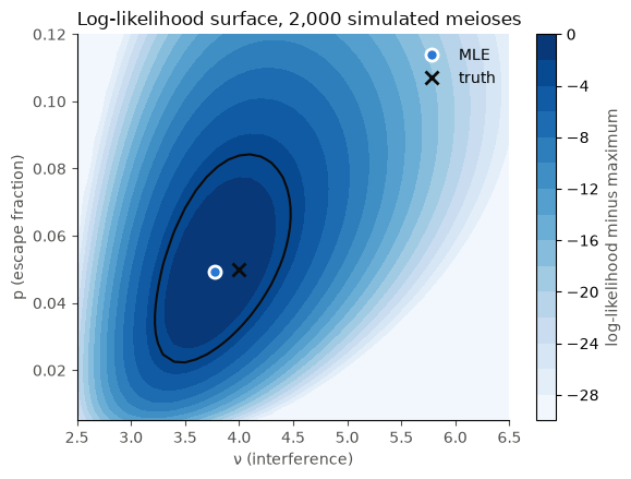
Likelihood surface

The log-likelihood relative to its maximum over a grid of \((\nu, p)\). The outlined region is the 95% joint confidence region (a drop of \(\chi^2_{2, 0.95}/2 \approx 3.0\) log-likelihood units). The region is tilted because the estimates of \(\nu\) and \(p\) are positively correlated: with more escape crossovers absorbing the close pairs, the remaining interference crossovers must be more regular, which means a larger \(\nu\).

nus = np.linspace(2.5, 6.5, 41)
ps = np.linspace(0.005, 0.12, 41)
surface = np.array([[loglik_fast(mz, None, nu=a, p=b, kernel=kernel) for a in nus] for b in ps])
rel = surface - ll_hat

ink, ink2, grid, accent = "#0b0b0b", "#52514e", "#e1e0d9", "#2a78d6"
fig, ax = plt.subplots(figsize=(6.4, 4.6))
levels = np.arange(-30, 0.1, 2.0)
filled = ax.contourf(nus, ps, np.maximum(rel, -30), levels=levels, cmap="Blues")
ax.contour(nus, ps, rel, levels=[-chi2.ppf(0.95, 2) / 2], colors=ink, linewidths=1.5, linestyles="solid")
ax.plot(nu_hat, p_hat, "o", ms=8, color=accent, mec="white", mew=2, label="MLE")
ax.plot(nu_true, p_true, "x", ms=9, mew=2, color=ink, label="truth")
cbar = fig.colorbar(filled, ax=ax)
cbar.set_label("log-likelihood minus maximum", color=ink2)
ax.set_xlabel("ν (interference)", color=ink2)
ax.set_ylabel("p (escape fraction)", color=ink2)
ax.set_title("Log-likelihood surface, 2,000 simulated meioses", color=ink, loc="left")
ax.legend(frameon=False, loc="upper right")
for side in ("top", "right"):
    ax.spines[side].set_visible(False)
ax.tick_params(colors=ink2)
plt.show()

Profile likelihood for \(\nu\)

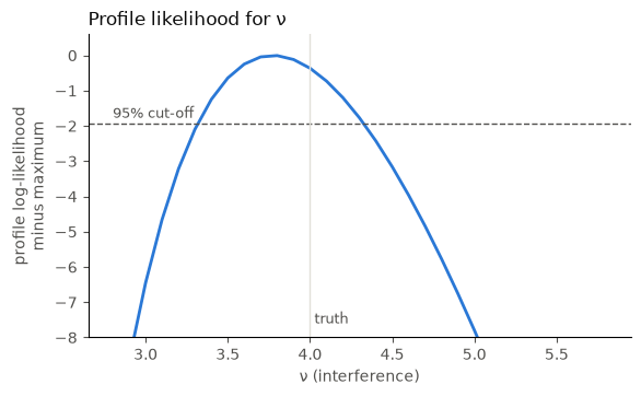
For each \(\nu\), maximise over \(p\). The interval where the profile is within \(\chi^2_{1, 0.95}/2 \approx 1.92\) of its maximum is a 95% profile-likelihood interval. It does not rely on the quadratic approximation behind the Wald interval, so the two can be compared.

def profile(nu):
    res = minimize(lambda t: -loglik_fast(mz, None, nu=nu, p=1 / (1 + np.exp(-t[0])), kernel=kernel),
                   x0=[fit.x[1]], method="Nelder-Mead", options=dict(xatol=1e-6, fatol=1e-8))
    return -res.fun


grid_nu = np.linspace(2.8, 5.8, 31)
prof = np.array([profile(v) for v in grid_nu]) - ll_hat
cut = -chi2.ppf(0.95, 1) / 2
inside = grid_nu[prof >= cut]
print(f"95% profile interval for nu: about [{inside.min():.2f}, {inside.max():.2f}] (grid step 0.1)")

fig, ax = plt.subplots(figsize=(6.4, 3.6))
ax.plot(grid_nu, prof, color=accent, lw=2)
ax.axhline(cut, color=ink2, lw=1, ls="--")
ax.text(grid_nu[0], cut + 0.15, "95% cut-off", color=ink2, fontsize=9)
ax.axvline(nu_true, color=grid, lw=1)
ax.text(nu_true, -7.6, " truth", color=ink2, fontsize=9)
ax.set_xlabel("ν (interference)", color=ink2)
ax.set_ylabel("profile log-likelihood\nminus maximum", color=ink2)
ax.set_title("Profile likelihood for ν", color=ink, loc="left")
ax.set_ylim(-8, 0.6)
for side in ("top", "right"):
    ax.spines[side].set_visible(False)
ax.tick_params(colors=ink2)
plt.show()

95% profile interval for nu: about [3.40, 4.30] (grid step 0.1)

Notes

• Per-meiosis parameters. nu and p may also be arrays with one value per meiosis, for example nu = np.exp(b0 + b1 * age). The same recipe then fits regression coefficients. With many distinct nu values the Chebyshev kernel falls back to the exact series.

• Phase-unknown data. For pooled crossovers from two meioses, replace loglik_fast with loglik_quartet; nothing else changes.

• Coordinates. Use genetic-map positions in Morgans. Physical positions would confound recombination hotspots with interference.